Basic statistics

 1 INTRODUCTION

This chapter will commence with an account of descriptive statistics, described by Battus (de Haan and van Hout 1986) as the useful loss of information. It also involves abstracting data. In any experimental situation we are presented with countable or measurable events such as the presence or degree of a linguistic feature in a corpus. Descriptive statistics enable one to summarise the most important properties of the observed data, such as its average or its degree of variation, so that one might, for example, identify the characteristic features of a particular author or genre. This abstracted data can then be used in inferential statistics (also covered in this chapter) which answers questions, formulated as hypotheses, such as whether one author or genre is different from another. A number of techniques exist for testing whether or not hypotheses are supported by the evidence in the data. Two main types of statistical tests for comparing groups of data will be described; i.e., parametric and non-parametric tests. In fact, one can never be entirely sure that the observed differences between two groups of data have not arisen by chance due to the inherent variability in the data. Thus, as we will see, one must state the level of confidence (typically 95 per cent) with which one can accept a given hypothesis.

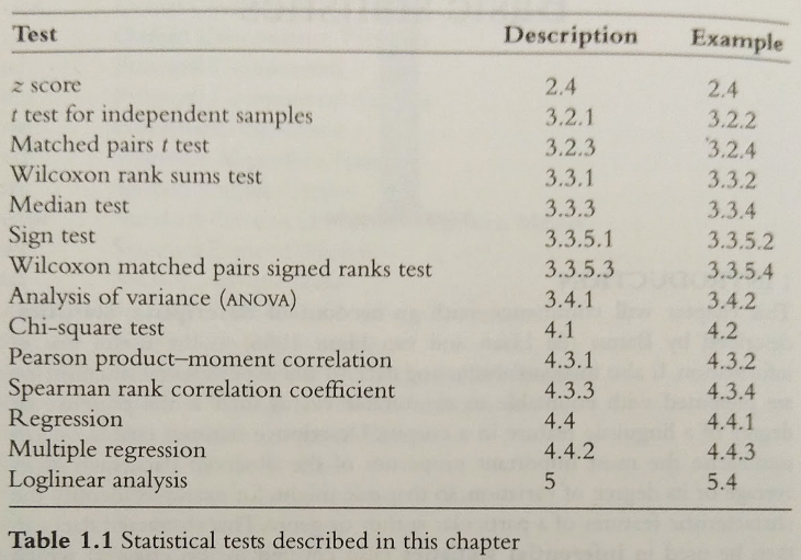
Correlation and regression are techniques for describing the relationships in data, and are used for answering such questions as whether high values of one variable go with high values of another, or whether one can predict the value of one variable when given the value of another. Evaluative statistics shows how a mathematical model or theoretical distribution of data relates to reality. This chapter will describe how techniques such as regression and loglinear analysis enable the creation of imaginary models, and how these are compared with real-world data from direct corpus analysis. Statistical research in linguistics has traditionally been univariate, where the distribution of a single variable such as word frequency has been studied. However, this chapter will also cover multivariate techniques such as ANOVA and multiple regress- ion which are concerned with the relationship between several variables. As each new statistical procedure is introduced, an example of its use in corpus linguistics will be given. A synopsis of the tests described in this chapter is given in Table 1.1.

This chapter will conclude with a description of Bayesian statistics, where we discuss our degree of belief in a hypothesis rather than its absolute probability.

2 DESCRIBING DATA

 2.1 Measures of central tendency

 The data for a group of items can be represented by a single score called a measure of central tendency. This is a single score, being the most typical score for a data set. There are three common measures of central tendency: the mode, the median and the mean. The mode is the most frequently obtained score in the data set. For example, a corpus might consist of sentences containing the following numbers of words: 16, 20, 15, 14, 12, 16, 13. The mode is 16, because there are more sentences with that number of words (two) than with any other number of words (all other sentence lengths occur only once). The disadvantage of using the mode is that it is easily affected by chance scores, though this is less likely to happen for large data sets.
 The median is the central score of the distribution, with half of the scores being above the median and half falling below. If there is an odd number of items in the sample the median will be the central score, and if there is an even Correlation and regression are techniques for describing the relationships in data, and are used for answering such questions as whether high values of one variable go with high values of another, or whether one can predict the value of one number of items in the sample, the median is the average of the two central scores. In the above example, the median is 15, because three of the sentences are longer (16, 16, 20) than this and three are shorter (12, 13, 14).
The mean is the average of all scores in a data set, found by adding up all the scores and dividing the total by the number of scores. In the sentence length example, the sum of all the words in all the sentences is 106, and the number of sentences is 7. Thus, the mean sentence length is 106/7 15.1 words. The = disadvantage of the mean as a measure of central tendency is that it is affected by extreme values. If the data is not normally distributed, with most of the items being clustered towards the lower end of the scale, for example, the median may be a more suitable measure. Normal distribution is discussed further in the section below.

2.2 Probability theory and the normal distribution

Probability theory originated from the study of games of chance, but it can be used to explain the shape of the normal distribution which is ubiquitous in nature. In a simple example, we may consider the possible outcomes of spinning an unbiased coin. The probability (p) of the coin coming up heads may be found using the formula p a/n where n is the number of equally = possible outcomes, and a is the number of these that count as successes. In the case of a two-sided coin, there are only two possible outcomes, one of which counts as success, so p = 1/2 = 0.5. The probability of the coin coming up tails (q) is also 0.5. Since heads and tails account for all the possibilities, p + q = 1; and as the outcome of one spin of the coin does not affect the outcome of the next spin, the outcomes of successive spins are said to be independent. For a conjunction of two independent outcomes, the probability of both occurring (p) is found by multiplying the probability of the first outcome p(a) by the probability of the second outcome p(b). For example, the probability of being dealt a queen followed by a club from a pack of cards would be 1/13 x 1/4 = 1/52. In the case of a coin being spun twice, the probability of obtaining two heads would be 1/2 x 1/2 = 1/4, and the probability of obtaining two tails would also be 1/4. The probability of obtaining a head followed by a tail would be 1/4, and that of obtaining a tail followed by a head would also be 1/4. Since there are two ways of obtaining one head and one tail (head first or tail first), the ratio of the outcomes no heads: one head:two heads is 1:2:1. Related ratios of possible outcomes for any number of trials (n) can be found using the formula (p + q) to the power n. If n is 3, we obtain p³ + 3p2q + 3pq² + q³. This shows that the ratio of times we get three heads:two heads: one head:no heads is 1:3:3:1. The number of times we expect to get r heads in n trials is called the binomial coefficient. This quantity, denoted by can also be found using the formula n!/r! (n-r)! where, for example, 4! means 44 x 3 x 2 x 1. The probability of success in a single trial is equal to

Plotting the probability values for all possible values of r produces the binomial probability graph.

Kenny (1982) states that any binomial distribution is completely described by p (probability) and n (number of trials). The mean is n x p, and the standard deviation is the square root of (n x px q), which is usually written as npq. The distribution is symmetrical if p and q are equally likely (equiprobable), as was the case for the coins, but skewed otherwise. When n is infinitely large, we obtain the normal distribution, which is a smooth curve rather than a frequency polygon. This curve has a characteristic bell shape, high in the centre but asymptotically approaching the zero axis to form a tail on either side. The normal distribution curve is found in many different spheres of life: comparing the heights of human males or the results of psychological tests, for example. In each case we have many examples of average scores, and much fewer examples of extreme scores, whether much higher or much lower than the average. This bell-shaped curve is symmetrical, and the three measures of central tendency coincide. That is to say, the mode, median and mean are equal. The normal distribution curve is shown in Figure 1.1(a). The importance of this discussion for corpus linguistics is that many of the statistical tests described in this chapter assume that the data are normally distributed. These tests should therefore only be used on a corpus where this holds true. An alternative type of distribution is the positively skewed distribution where most of the data is bunched below the mean, but a few data items form a tail a long way above the mean. In a negatively skewed distribution the converse is true; there is a long tail of items below the mean, but most items are just above it. The normal distribution has a single modal peak, but where the frequency curve has two peaks bimodal distributions also occur. Figure 1.1(b) shows a positively skewed distribution, Figure 1.1(c) shows a negatively skewed distribution and Figure 1.1(d) shows a bimodal distribution.
In corpus analysis, much of the data is skewed. This was one of Chomsky's main criticisms of corpus data, as noted by McEnery and Wilson (1996). For example, the number of letters in a word or the length of a verse in syllables are usually positively skewed. Part of the answer to criticism of corpus data based on the 'skewness' argument is that skewness can be overcome by using lognormal distributions. For example, we can analyse a suitably large corpus according to sentence lengths, and produce a graph showing how often each sentence length occurs in the corpus. The number of occurrences is plotted on the vertical (y) axis, and the logarithm of the sentence length in words is plotted along the horizontal (x) axis. The resulting graph will approximate to the normal distribution. Even when data is highly skewed, the normal curve is