고정 헤더 영역
상세 컨텐츠
본문

반응형
Abstract
Political scientists often cite the importance of mechanism-specific causal knowledge, both for its intrinsic scientific value and as a necessity for informed policy. This article explains why two common inferential heuristics for mechanism-specific (i.e., indirect) effects can provide misleading answers, such as sign reversals and false null results, even when linear regressions provide unbiased estimates of constituent effects. Additionally, this article demonstrates that the inferential difficulties associated with indirect effects can be ameliorated with the use of stratification, interaction terms, and the restriction of inference to subpopulations (e.g., the indirect effect on the treated). However, indirect effects are inherently not identifiable—even when randomized experiments are possible. The methodological discussion is illustrated using a study on the indirect effect of Islamic religious tradition on democracy scores (due to the subordination of women).
The explicit or implicit focus on indirect effects (sometimes known as path specific effects, or causal mechanisms,1 or mediation analysis) pervades important topics across all empirical subfields of political science:
We wish to account for a single behavior at a fixed point in time. But it is behavior that stems from a multitude of prior factors. We can visualize the chain of events with which we wish to deal as contained in a funnel of causality. (Campbell et al. 1960, 24)
I do not model presidential election rules as having a direct impact on the legislative party system. Instead, there is a two-step process: (1) Presidential election rules combine interactively with social diversity to produce an effective number of presidential candidates; (2) the effective number of presidential candidates affects the effective number of legislative competitors. … (Cox 1997, 204)
The hypothesis we are interested in is that β= 0; that is, population density or urbanization in 1500 affects income today only via institutions. (Acemoglu et al. 2002, 1269)
The empirical pattern is thus inconsistent with H1, the common expectation that ethnic diversity is a major and direct cause of civil violence. Nor is there strong evidence in favor of H2, which expects ethnic strife to be activated as modernization advances. Ethnic diversity could still cause civil war indirectly, if it causes lower per capita income (Easterly and Levine 1997) or a weak state. (Fearon and Laitin 2003, 82)
In short, because researchers often want to describe how a cause affects an outcome, the importance of indirect effects is now taken as given. It is not generally understood how difficult it is to gain such knowledge.
Although it is well known that the assumptions necessary for the exact estimation of indirect effects via path analysis are rarely satisfied (Baron and Kenny 1986; Duncan 1985; Goldberger 1972; Haavelmo 1943; Simon 1953), the rules of path analysis are often used implicitly as heuristics—a product heuristic and a difference heuristic—within regression tables. The product heuristic can be stated as the following—if regressions (with control variables) provide evidence for the effect of A on B and the effect of B on C, then the indirect effect of A on C that goes through B is roughly the product of the effect of A on B and the effect of B on C.

The difference heuristic can be stated as the following—if regressions (with control variables) provide evidence for the total effect of A on C and the direct effect of A on C once we have controlled for the effect of B on C, then the indirect effect of A on C that goes through B is roughly the difference between these effects.
Readers familiar with standard regression practice will notice that the difference heuristic is often utilized when regression coefficients are compared across different regression specifications with the same outcome variable, and the product heuristic is often utilized when regression evidence is combined across regressions with different outcome variables. Such heuristic reasoning with regression tables is so pervasive within the social science literature that examples are too numerous to cite. Baron and Kenny (1986), the paper that largely established the use of these techniques, has been cited more than 20,000 times. Furthermore, as the above quotes indicate, some of the most influential work in political science utilizes these heuristics—including two of the most cited papers of the last decade (both with more than 1,500 citations).2
These heuristics would not be especially problematic if they rarely produced unreasonable inferences. However, as with other fallacies of inference, such as the ecological fallacy (Robinson 1950), the conditions under which the product and difference heuristics will produce misleading results are quite common. As with the ecological fallacy, when parameters vary across the units of analysis, the product and difference heuristics can produce false positive results, false null results, or results with the wrong sign—even when linear models are appropriate. Furthermore, most theories in political science predict that parameters will vary across the units of analysis. We would hardly expect different political actors to respond in a homogenous manner to causes (e.g., registration laws affect politically active individuals differently than they affect politically inactive individuals and close elections affect recently established democracies differently than they affect long-established democracies). In political science applications, causal effect heterogeneity is the rule, not the exception.
The crux of the problem can be understood with a stylized example. Suppose we were able to randomly assign A in a very large sample, or we were able to control for enough covariates that we believed we had approximated the random assignment of A. Suppose further that when we regressed B on A, we found that A had no effect on B (the coefficient was zero with a very small standard error). It seems logical to take this as sufficient evidence that there is no indirect effect of A through B on C because in order for this effect to be present, surely A must affect B. However, this reasoning is fallacious because when causal effects are heterogeneous, randomized experiments identify average effects but not individual effects. This is also true of techniques such as multiple regression or matching that attempt to approximate randomized experiments.
To see the difficulty, suppose that the effect of A on B is positive for half of the individuals in the study and the effect of A on B is negative for the other half of the individuals in the study. In this case, we might estimate an effect of zero because these effects would cancel with each other. Furthermore, if the effect of B on C is positive for the individuals for whom the effect of A on B is positive, and the effect of B on C is negative for the individuals for whom the effect of A on B is negative, then the indirect effect is positive for all individuals. Therefore, it is possible for the average effect of A on B to be zero while the indirect effect of A through B on C is positive for everyone. The remainder of this article merely demonstrates that fallacies of this type have serious consequences for the study of indirect effects and causal mechanisms within political science.
This is not the first article to note the difficulties that effect heterogeneity creates for making inferences about indirect effects. These difficulties have been documented at least since Robins and Greenland (1992). However, despite the warnings presented in that article, the special conditions required for valid inferences about indirect effects are almost never discussed explicitly within the political science literature.
This article explains the difficulties of inference for indirect effects by providing a stylized and intuitive presentation within the familiar context of linear models for cross-sectional data. The simplification to cross-sectional linear models focuses attention on the extra difficulties associated with indirect effects. In addition, the simplification to linear models allows a decomposition of direct and indirect effects that closely resembles the traditional path analytic decomposition, and this decomposition allows the comparison of differing identification criteria for average indirect effects (Imai et al. 2010d; Pearl 2001; Petersen et al. 2006; Robins 2003; Robins and Greenland 1992). The methodological points of this article are illustrated with an example from the literature on the democracy deficit for Muslim countries. The use in this example of cross-sectional linear models, a binary explanatory variable, and a single control variable greatly simplifies the discussion.
This article is organized as follows. The next section describes the source of the product and difference heuristics within the context of linear constant-effects models. This is followed by a section demonstrating that the product heuristic can be misleading if effects are heterogeneous, and then a section demonstrating that the difference heuristic can be misleading if there are also interactions between the explanatory variable and the intermediate variable. The final sections discuss indirect effects for subpopulations (e.g., the average indirect effect on the treated) and suggestions for future research practice.
The Source of the Product and Difference Methods
Before describing the situations in which the product and difference methods fail, it will be useful to describe the situation in which these methods succeed. With this goal in mind, we assume a simple linear path model with constant effects for independent observations indexed by i= 1, … , n. In this model (depicted graphically in Figure 1(a)) the explanatory variable Xi may affect both the intermediate/mediating variable Zi and the outcome variable Yi, and the intermediate variable Zi may also affect the outcome variable. In order to be explicit about the definition of indirect effects, we will write this model with potential outcomes notation as the following:
Here, Zi(x) represents the potential value of the mediator for individual i if Xi is set to take the value x, and Yi(x, z) is the joint potential outcome for individual i if Xi is set to take the value x and Zi is set to take the value z. These potential outcomes and mediators are assumed to be well defined for all possible values of x and z (i.e., SUTVA [Angrist et al. 1996] holds) in the sense that Zi(x) and Yi(x, z) are individual specific functions. For this particular model, all individual specific functions are linear in x and z and the only aspects of the functions that vary across individuals are the “error terms” (δi and εi), which can be interpreted as individual-level shifts in the intercept. We are agnostic as to the distribution of these “error terms” within the population. In later sections of the article, other aspects of the functions will be allowed to vary across individuals.
Using this notation, the observed mediator can be written as Zi=Zi(Xi), and the observed outcome can be written as Yi=Yi(Xi, Zi(Xi)). With this model and notation, we can define the reduced-form potential outcomes and model recursively,
and the total effects can be defined as a change in the explanatory variable that is allowed to propagate through both the direct and indirect channels.
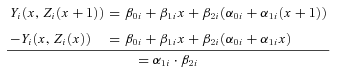
Note that the second term in (3) can be interpreted as an indirect effect because it corresponds to be the change we would see if the explanatory variable had an effect on the intermediate variable, but not directly on the outcome variable (Yi(x, Zi(x+ 1)) −Yi(x, Zi(x))):
Note further that this indirect effect is the product of the effect of the explanatory variable on the intermediate variable and the effect of the intermediate variable on the outcome.
Therefore, if we further assume that a regression of Z on X and other control variables will provide an unbiased estimate of α1 and a regression of Y on Z and X and other control variables will provide an unbiased estimate of β2, then we may consistently estimate the indirect effect with the product of these two estimates.3
Furthermore, if we assume that we can obtain an unbiased estimate of β1+β2·α1 with a regression of Y on X and other control variables, and we can obtain an unbiased estimate of β1 with a regression of Y on X and Z and other control variables, the difference of these two estimates provides an unbiased estimate of the indirect effect. Therefore, in this model (linear with constant effects), the product and difference heuristics work perfectly.
Of course, it is well known that these product and difference methods do not provide consistent estimates for more complicated models. However, in more complicated settings, these two methods are often used as heuristics because it is frequently assumed that they will produce estimates with the correct sign and/or approximately the correct magnitude. In the following two sections, I explain why the product and difference heuristics can produce highly misleading answers, such as sign reversals and false null results, as soon as we allow for heterogeneous effects and interactions.
The Product Fallacy
Suppose we assume a linear path model with heterogeneous effects but no individual-level interactions between the explanatory variable and the intermediate variable.
Note that error terms are redundant in this model (α0i≡α*0i+δi and β0i≡β*0i+εi), so they have been removed from the notation. Note as well that the only difference between this model and the model in the previous section is that α1i, β1i, β2i now have i subscripts. This indicates that X is allowed to have different effects on Z for each individual, and X and Z are allowed to have different effects on Y for each individual. Finally, note that this model is consistent with various hierarchical or multilevel models, but we are agnostic as to the distribution of α1i, β1i, β2i (conditional on Xi, Zi, and Yi).
As in (4), we can define the individual-level indirect effect to be the change we would see if the explanatory variable had an effect on the intermediate variable, but not directly on the outcome variable.
Note that the individual-level indirect effect is still the product of the individual-level effect of the explanatory variable on the intermediate variable and the individual-level effect of the intermediate variable on the outcome. However, these indirect effects and their components (α1i and β2i) are heterogeneous across individuals.4
In heterogeneous effects models like this, regressions will not generally provide estimates of the individual effects (Holland 1986), so that even random assignment of the explanatory variable only identifies average effects. However, even if we assume that a regression of Z on X and other control variables provides an unbiased estimate of

and a regression of Y on Z and X and other control variables provides an unbiased estimate of

, and even if we restrict our attention to the average indirect effect (

), the product heuristic can provide highly misleading estimates. This is because an average of products is equal to a product of the constituent averages plus the covariance between the constituents,

where

. Therefore, if the effect of X on Z is highly correlated (positively or negatively) with the effect of Z on Y, then the product heuristic can produce false null results or even results with the wrong sign.
Unfortunately, because regressions do not produce individual-level effect estimates, the covariance term in (8) cannot be identified and can therefore never be accounted for completely. However, partial tests may be available, and some values of Cov(α1, β2) will be more plausible than others. This will be easier to discuss in the context of an example.
An Example Illustrating the Product Fallacy
In an important and highly cited paper on Islam and authoritarianism, Fish (2002) presents cross-national evidence that countries with an Islamic religious tradition tend to have more authoritarian governments. Furthermore, this paper uses the product heuristic a number of times to argue that this relationship may be partially due to the subordination of women within predominantly Muslim societies (societies with an Islamic religious tradition).
For example, this paper presents a regression of country-level sex ratios (number of men per 100 women) on country-level income and on an indicator for Islamic religious tradition (IRT)—as evidence for a positive effect of IRT on sex ratios. This paper also presents a regression of Freedom House (FH) democracy scores (reversed so that higher scores indicate more democratic countries) on income, IRT, and sex ratio—as evidence for a negative effect of sex ratios on democracy scores:
...the difference in sex ratios between Muslim and Catholic countries is large and statistically significant, as is the difference between Muslim and all non-Muslim countries. Models 3 and 4 in Table 9 show this finding. Table 10 shows that in a regression using FH scores as the dependent variable, sex ratio differences are statistically significant even when controlling for Islam and level of development. (Fish 2002, 28)
Are these results—a significant Muslim versus non-Muslim effect on sex ratio and a significant sex ratio effect on FH scores—convincing evidence for the indirect effect of IRT on democracy due to female subordination? As in all observational studies, we might worry that the correct variables have not been measured (or have been measured incorrectly).5 We might worry about balance and overlap. We might worry that functional form assumptions are not appropriate. However, the fundamental problem of indirect effects is that, even if the above cited results are robust to all of these concerns, the implied indirect effect is not robust without additional assumptions.6
As a stylized example, suppose there are two types of countries. The first type has a high sex ratio if and only if it has an Islamic religious tradition (α1i > 0), but sex ratio has little effect on its democracy score (β2i≈ 0). The indirect effect is approximately zero for this type of country (α1i·β2i≈ 0). For the second type of country, Islamic religious tradition has little effect on sex ratio (α1i≈ 0), but sex ratio negatively affects the democracy score (β2i < 0). The indirect effect is also approximately zero for this type of country (α1i·β2i≈ 0). Furthermore, if the population is composed of equal amounts of these two types of countries, then the average effect of Islamic religious tradition on sex ratio is positive (

), and the average effect of sex ratio on democracy score is negative (

). Therefore, the product method (

) would suggest that the average indirect effect is negative, when in fact the indirect effect is essentially zero for all countries. The fallacy occurs in this case because the covariance between the two effects is positive (Cov(α1, β2) > 0), and this cancels with the negative estimate from the product method.
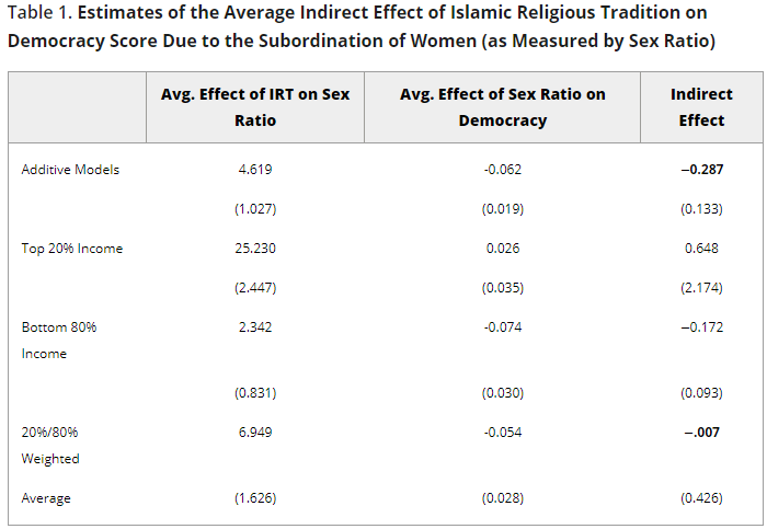
Unfortunately, we cannot estimate the covariance between the effects. However, if we have a theoretical reason to believe that the magnitude of the covariance might be smaller within levels of stratification, then we may be able to ameliorate the effects of this covariance. For example, consider the evidence cited in Fish (2002), reproduced here in the first row of Table 1.7 Within these additive linear models, the average effect of IRT on sex ratio(

) is estimated to be 4.619, and the average effect of sex ratio on democracy score (

) is estimated to be −0.062. Using the product method, this implies an estimated average indirect effect of −0.287. However, although these models control for income in an additive manner, we might worry that there is positive correlation between the IRT and sex ratio effects, and furthermore, we might think that this covariance will be smaller within levels of income.As a first test, suppose that instead of conditioning on income in an additive model, we split the sample into high-income countries (countries above the upper quintile) and lower-income countries (countries below the upper quintile). Rows 2 and 3 of Table 1 show that when we regress sex ratio on IRT among the high-income countries, we estimate an IRT effect of 25.230, and when we regress sex ratio on IRT among the lower-income countries, we estimate an IRT effect of 2.342. However, even though we find evidence of heterogeneity, it is important to note that this stratification does not substantially change our impression of the original estimate of

. To see this, note that when we average these two effects according to the proportion of high- and lower-income countries (Row 4 of Table 1), we estimate the average effect of IRT on sex ratio (

) to be .2 · 25.23 + .8 · 2.342 = 6.949. Therefore, the estimate of 4.619 for the positive IRT effect is robust to the use of this interaction model (in fact, the estimated

increases by roughly 50%).
As a first test, suppose that instead of conditioning on income in an additive model, we split the sample into high-income countries (countries above the upper quintile) and lower-income countries (countries below the upper quintile). Rows 2 and 3 of Table 1 show that when we regress sex ratio on IRT among the high-income countries, we estimate an IRT effect of 25.230, and when we regress sex ratio on IRT among the lower-income countries, we estimate an IRT effect of 2.342. However, even though we find evidence of heterogeneity, it is important to note that this stratification does not substantially change our impression of the original estimate of
. To see this, note that when we average these two effects according to the proportion of high- and lower-income countries (Row 4 of Table 1), we estimate the average effect of IRT on sex ratio (
) to be .2 · 25.23 + .8 · 2.342 = 6.949. Therefore, the estimate of 4.619 for the positive IRT effect is robust to the use of this interaction model (in fact, the estimated
increases by roughly 50%).As a first test, suppose that instead of conditioning on income in an additive model, we split the sample into high-income countries (countries above the upper quintile) and lower-income countries (countries below the upper quintile). Rows 2 and 3 of Table 1 show that when we regress sex ratio on IRT among the high-income countries, we estimate an IRT effect of 25.230, and when we regress sex ratio on IRT among the lower-income countries, we estimate an IRT effect of 2.342. However, even though we find evidence of heterogeneity, it is important to note that this stratification does not substantially change our impression of the original estimate of
. To see this, note that when we average these two effects according to the proportion of high- and lower-income countries (Row 4 of Table 1), we estimate the average effect of IRT on sex ratio (
) to be .2 · 25.23 + .8 · 2.342 = 6.949. Therefore, the estimate of 4.619 for the positive IRT effect is robust to the use of this interaction model (in fact, the estimated
increases by roughly 50%).
Similarly, when we regress democracy scores on sex ratio and IRT among the high-income countries, we estimate a sex ratio effect of 0.026, and when we regress democracy scores on sex ratio and IRT among the lower-income countries, we estimate a sex ratio effect of −0.074—again some evidence of an interaction. However, as before when we average these two effects according to the proportion of high- and lower-income countries, we estimate the average effect of sex ratio on democracy (

) to be .2 · 0.026 + .8 · (−0.074) =−0.054. Therefore, the estimate of −0.062 for the negative sex ratio effect is robust to the use of this interaction model (although the magnitude of the effect decreases slightly). Finally, notice that the product of our new estimates for

and

actually implies a more substantial indirect effect (6.95 ×−0.054 =−0.373).
We might take the robustness of the estimates for these two effects (

and

) to imply robustness for our estimated indirect effect. However, the robustness of these constituent effects does not transfer to the average indirect effect. Rows 2 and 3 of Table 1 demonstrate that the estimated indirect effect (taking the products within rows) is 0.648 for high-income countries and −0.172 for low-income countries (note that these estimates do not bracket the original estimate of −0.287). When averaged according to the proportions of high- and lower-income countries, we see that the average indirect effect is effectively zero (.2 · 0.648 + .8 · (−0.172) =−0.007). In other words, even if the estimated effects of IRT on sex ratio (

) and sex ratio on democracy (

) are robust, the estimated average indirect effect (

) is not robust. Notice that this lack of robustness is due to positive covariance between the constituent effects. Both of the effects are larger for the high-income group and lower for the low-income group. This positive covariance cancels with the negative effect produced by the product heuristic and results in an estimate near zero.
Of course, this analysis should not be taken as definitive. Stratification on other variables might restore the negative indirect effect or might even produce a positive indirect effect. What this example demonstrates is the additional burden associated with the use of the product method for the estimation of indirect effects—it is not enough to provide robust estimates of the constituent average effects. In addition to the usual task incumbent on the analyst—arguing that the two regression coefficients approximate results from randomized experiments—the analyst must also argue that the covariance between the individual-level constituent effects is minimal. In other words, the analyst must argue that conditions hold in addition to those that would be justified by randomized experiments.Therefore, if we can somehow obtain an unbiased estimate of

with a regression of Y on X and other control variables, and an unbiased estimate of

with a regression of Y on X and Z and other control variables, the difference of these two estimates provides an unbiased estimate of the average indirect effect.

The Difference Fallacy
Given the difficulties of the product method, we might instead rely on the difference method. Using the model in (5) and (6), we can again define the total effects as a change in the explanatory variable that is allowed to propagate through both the direct and indirect channels.

Therefore, if we can somehow obtain an unbiased estimate of
with a regression of Y on X and other control variables, and an unbiased estimate of
with a regression of Y on X and Z and other control variables, the difference of these two estimates provides an unbiased estimate of the average indirect effect.
However, if there is an individual-level interaction between the explanatory variable and the intermediate variable,


the definition of direct and indirect effects becomes more complicated, and the difference method can produce misleading results.
Defining Indirect Effects in the Interaction Model
For this interaction model with heterogeneous effects, there are many possible indirect effects. Recall that in the constant effects model (4) and in the heterogeneous effects model without an interaction (7), the indirect effect was defined as Yi(x, Zi(x+ 1)) −Yi(x, Zi(x)). With an interaction between the explanatory and intermediate variables, this indirect effect becomes
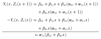
However, while the indirect effects in the non-interaction models ((4) and (7)) are equal regardless of the fixed value of the explanatory variable (e.g., Yi(x, Zi(x+ 1)) −Yi(x, Zi(x)) =Yi(x+ 1, Zi(x+ 1)) −Yi(x+ 1, Zi(x))), for the interaction model, these indirect effects are not equal:
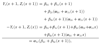
where (12) is not equal to (13). Therefore, we have at least two parameters of potential interest from our analysis,


반응형
'Political Science' 카테고리의 다른 글
| Islam, Authoritarianism, and Female Empowerment: What Are the Linkages? (0) | 2022.10.04 |
|---|---|
| The Product and Difference Fallaciesfor Indirect Effects(2/2) (0) | 2022.10.04 |
| Playing to the Gallery: Emotive Rhetoric in Parliaments (0) | 2022.09.28 |
| WHAT DEMOCRACY IS . . . AND IS NOT (0) | 2022.09.25 |
| Web-Based Survey Methodology (0) | 2022.09.25 |


